TP de conception d'un filtre de signaux ECG
VHDL Cheat
https://memo-vhdl.gitlab-pages.imt-atlantique.fr/
Dépôt Gitlab associé
Un dépôt gitlab tp-ecg-etudiant est disponible dans votre espace gitlab sur https://gitlab-df.imt-atlantique.fr, dans le groupe correspondant à l'enseignement suivi.
Pour le manipuler (clone, add, commit, push, pull), veuillez vous référer à la page Git et Gitlab .
Objectifs
Pour analyser des signaux physiologiques échantillonnés, il faut d ́abord les traiter pour supprimer plusieurs sources de bruit, des artefacts et autres signaux parasites. Le traitement numérique est particulièrement intéressant pour sa capacité à être finement adapté au cas considéré. A titre d’exemple, nous allons considérer le traitement de signaux de type électrocardiogramme (ECG).
Sur la base PhysioNet (https://www.physionet.org/), nous trouvons plusieurs jeux de données de différents types de signaux, dont des ECG (https://www.physionet.org/about/database/#ecg) échantillonnés dans diverses conditions.
Il est simple d’accéder à différents fichiers dans différents formats sur l’archive de PhysioNet (https://archive.physionet.org/cgi-bin/atm/ATM). Pour vos travaux, nous proposons sur Moodle un ficher CSV issu de la base MIT-BIH Arrhythmia, avec un signal échantillonné à 500Hz (fréquence de Nyquist = 250Hz) et codé sur 11 bits en entiers dans le fichier retenu.
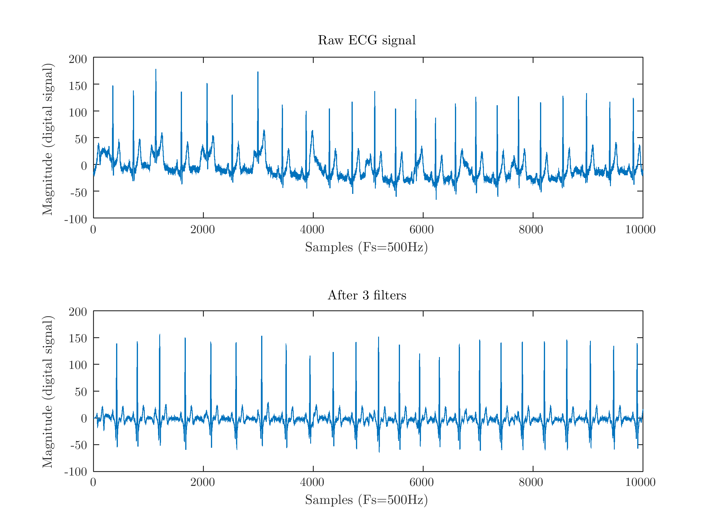
Lorsque l’on affiche le signal numérique brut et ce que l’on peut obtenir après trois filtrages (une suppression de la ligne de base isoélectrique, du bruit d’alimentation (50 ou 60 Hz selon le pays où sont réalisées les mesures et du bruit à haut fréquence), on observe clairement un avantage à traiter le signal pour permettre une analyse des mesures par un praticien.
Le code Octave (alternative libre à Matlab, disponible sur les machines Linux de l’École) qui permet d’effectuer ces traitements est disponible à la section Code Octave du filtrage par trois filtre successifs:
Il est disponible dans le dépôt tp-ecg-etudiant au chemin src-ref/octaveScript.m.
Vous noterez que ce script finit par l’appel d’une fonction de la littérature , qui fournit un code inclus en annexe de ce document.
C’est un fichier de référence pour une première découverte de traitements classiques et simples d’ECG, exploitant le très connu algorithme de PAN-TOMPKINS qui fut publié en 1985 et intégré par la suite dans de nombreux dispositifs commerciaux. Évidemment, l’état de l’art offre des performances supérieures mais requiert des connaissances et compétences nécessitant plusieurs dizaines d’heures d’apprentissage.
Travail attendu
Un dépôt git a été créé pour chaque étudiant sur l'instance gitlab de la DFVS de l'école https://gitlab-df.imt-atlantique.fr. Il contient les sources VHDL nécessaires au projet, des scripts pour gérer le projet Vivado, et un compte-rendu.md permettant de répondre aux questions. Si vous travaillez en binôme, choisissez un des deux, et ajoutez votre collègue en tant que owner sur le projet dans gitlab.
Warning
Pensez à adapter le chemin de la commande ci-dessous à vos propres besoins
| mkdir -p ~/chemin/souhaite/tp-vhdl-mee/nom-de-UE/
cd !$
|
- Clonage en local du dépôt git
Warning
Pensez à adapter le chemin de la commande ci-dessous à vos propres besoins
| git clone https://gitlab-df.imt-atlantique.fr/tp-vhdl-mee/medcon/gr-vhdl-$USER/tp-filtre-etudiant-$USER.git
|
git clone permet de récupérer l'entièreté du dépôt git avec son historique de modifications.
Vous pouvez observer facilement ce cette commande a permit de télécharger avec la commande ls -alsh dans le répertoire tp-ecg-etudiant-$USER.
Création d’un projet Vivado
Warning
Ne mettez jamais d'espaces, d'accent ni de caractères spéciaux dans les noms de fichiers ou de répertoires ! Ceci est valable en général, sur Windows comme sur Linux. Et fait planter Vivado en ce qui nous concerne ici.
Retour au répertoire racine utilisateur et lancement de Vivado 2020.2 :
| cd
SETUP MEE_VITIS20202 && vivado &
|
Dans le temps imparti, nous vous suggérons d’intégrer, sur la base de l’architecture de filtre décrite dans le chapitre précédent, le pré-traitement des méthodes proposées.
Soit :
- vous intégrez un banc de filtres programmables qui permet de réaliser les trois premiers filtres du script (suppression de la ligne de base, élimination du bruit à 50Hz par un coupe-bande tout basique ou Pei-Tseng, lissage du bruit haute fréquence par filtre de Parks-McClellan) en temps réel
-
soit vous intégrez la phase de pré-traitement de l’algorithme de PAN-TOMPKINS. Celle-ci est constituée de :
-
un filtre passe-bas dans la bande 5-15Hz
- un filtre dérivatif pour mettre en évidence le complexe QRS qui sert au diagnostic
- une élévation au carré du signal
- un moyennage pour supprimer le bruit haute fréquence (sur une durée de 150ms).
Le code de cet algorithme est disponible à la section Code octave de l'algorithme de PAN-TOMPKINS
Question
Le travail à fournir, outre la description VHDL et les différents tests en simulation consiste à
- concevoir une architecture d'unité opérative, grâce au fichier disponible dans le dépôt tp-ecg-etudiant au chemin
docs/img/OperativeUnit.drawio, modifiable avec l'outil en ligne Draw.io : https://app.diagrams.net/
- concevoir une FSM correspondante via le fichier
docs/img/FSM.drawio.
- exporter vos schémas au formats
PNG, avec les noms OperativeUnit.png et FSM.png
- compléter le squelette de compte rendu disponible dans
docs/compte-rendu.md avec toute information que vous jugerez nécessaire.
Votre circuit doit pouvoir fournir un pré-traitement le plus rapidement possible à une unité plus complexe qui surveillera en permanence et en temps réel l’état de santé d’un patient. Par conséquent, votre travail sera évalué sur la base de votre capacité à décrire un circuit qui réalise en temps réel le pré-traitement attendu avec fidélité (précision équivalente) et le minimum possible de ressources matérielles. Votre prototypage se fera dans un environnement FPGA, que nous pourrons connecter à une carte fille d’extraction de signal ECG.
Code Octave du filtrage par trois filtre successifs
| Code Octave de filtrage d'ECG |
|---|
1
2
3
4
5
6
7
8
9
10
11
12
13
14
15
16
17
18
19
20
21
22
23
24
25
26
27
28
29
30
31
32
33
34
35
36
37
38
39
40
41
42
43
44
45
46
47
48
49
50
51
52 | % ECG telecharge de
%https://archive.physionet.org/cgi-bin/atm/ATM
%Echantillonne à 500Hz (F_Nyquist = 250Hz)
% Script OCTAVE (pas matlab...)
Fs = 500; % Frequence d'echantillonnage
Fn = Fs/2; % Frequence de Nyquist
figure(1)
T = csvread('./ADCSamplesOctave.csv');
subplot(2,3,1);plot(T(:,2));title('Raw ECG signal');xlabel('Samples (Fs=500Hz)');ylabel('Magnitude (output of an 11-bit ADC)');
% Pourc Octave (a supprimer sous Matlab)
pkg load signal;
%Pour les trois filtres suivants, on peut jouer sur les ordres
% donc le nombre de coefficients des filtres numeriques
%suppression de la baseline
fBaseLine=fir1(128, 5/Fn, 'high');
y_minus_BL=filter(fBaseLine,[1],T(:,2));
subplot(2,3,2);plot(y_minus_BL);title('Baseline wander reduced');xlabel('Samples (Fs=500Hz)');ylabel('Magnitude (digital signal)');
subplot(2,3,3);plot(y_minus_BL(1:1000));title('Baseline wander reduced -- zoomed');xlabel('Samples (Fs=500Hz)');ylabel('Magnitude (digital signal)');
%elimination du bruit à 50Hz par un coupe-bande tout basique
f50Hz=fir1(100, [45 55]/Fn, 'stop');
y_minus_50Hz_simple = filter(f50Hz,[1],y_minus_BL);
subplot(2,3,4);plot(y_minus_50Hz_simple(1:1000));title('FIR1 band-cut-- zoomed');xlabel('Samples (Fs=500Hz)');ylabel('Magnitude (digital signal)');
%elimination du bruit à 50Hz par un coupe-bande plus elabore
[b,a]=pei_tseng_notch ( 50 / Fn, 10/Fn );
y_minus_50Hz_pei_tseng = filter(b,a,y_minus_BL);
subplot(2,3,5);plot(y_minus_50Hz_pei_tseng(1:1000));title('Pei Tseng band-cut -- zoomed');xlabel('Samples (Fs=500Hz)');ylabel('Magnitude (digital signal)');
%lissage du bruit haute frequence par filtre de Parks-McClellan
Fpass = 50;
Fstop = 60;
F = [0 Fpass Fstop Fn]/(Fn);
A = [1 1 0 0];
fLP = remez(10,F,A); % Voir pour Matlab: firpm
yLP = filter(fLP,[1],y_minus_50Hz_pei_tseng);
subplot(2,3,6);plot(yLP(1:1000));title('Low-pass filter to suppress high-freq noise -- zoomed');xlabel('Samples (Fs=500Hz)');ylabel('Magnitude (digital signal)');
figure(2)
subplot(2,1,1);plot(T(:,2));title('Raw ECG signal');xlabel('Samples (Fs=500Hz)');ylabel('Magnitude (digital signal)');
subplot(2,1,2);plot(yLP);title('After 3 filters');xlabel('Samples (Fs=500Hz)');ylabel('Magnitude (digital signal)');
print(2, "ECG_raw_3filters.pdf", "-dpdflatexstandalone");
figure(3)
%L'artillerie lourde: fonction intégrant la methode de Pan-Tompkin
%merci Sedghamiz. H !!!
pan_tompkin(T(:,2),500,1)
|
Code octave de l'algorithme de PAN-TOMPKINS
| Code Octave de l'algorithme de PAN-TOMPKINS |
|---|
1
2
3
4
5
6
7
8
9
10
11
12
13
14
15
16
17
18
19
20
21
22
23
24
25
26
27
28
29
30
31
32
33
34
35
36
37
38
39
40
41
42
43
44
45
46
47
48
49
50
51
52
53
54
55
56
57
58
59
60
61
62
63
64
65
66
67
68
69
70
71
72
73
74
75
76
77
78
79
80
81
82
83
84
85
86
87
88
89
90
91
92
93
94
95
96
97
98
99
100
101
102
103
104
105
106
107
108
109
110
111
112
113
114
115
116
117
118
119
120
121
122
123
124
125
126
127
128
129
130
131
132
133
134
135
136
137
138
139
140
141
142
143
144
145
146
147
148
149
150
151
152
153
154
155
156
157
158
159
160
161
162
163
164
165
166
167
168
169
170
171
172
173
174
175
176
177
178
179
180
181
182
183
184
185
186
187
188
189
190
191
192
193
194
195
196
197
198
199
200
201
202
203
204
205
206
207
208
209
210
211
212
213
214
215
216
217
218
219
220
221
222
223
224
225
226
227
228
229
230
231
232
233
234
235
236
237
238
239
240
241
242
243
244
245
246
247
248
249
250
251
252
253
254
255
256
257
258
259
260
261
262
263
264
265
266
267
268
269
270
271
272
273
274
275
276
277
278
279
280
281
282
283
284
285
286
287
288
289
290
291
292
293
294
295
296
297
298
299
300
301
302
303
304
305
306
307
308
309
310
311
312
313
314
315
316
317
318
319
320
321
322
323
324
325
326
327
328
329
330
331
332
333
334
335
336
337
338
339
340
341
342
343
344
345
346
347
348
349
350
351
352
353
354
355
356
357
358
359
360
361
362
363
364
365
366
367
368 | function [qrs_amp_raw,qrs_i_raw,delay]=pan_tompkin(ecg,fs,gr)
%% function [qrs_amp_raw,qrs_i_raw,delay]=pan_tompkin(ecg,fs)
% Complete implementation of Pan-Tompkins algorithm
%% Inputs
% ecg : raw ecg vector signal 1d signal
% fs : sampling frequency e.g. 200Hz, 400Hz and etc
% gr : flag to plot or not plot (set it 1 to have a plot or set it zero not
% to see any plots
%% Outputs
% qrs_amp_raw : amplitude of R waves amplitudes
% qrs_i_raw : index of R waves
% delay : number of samples which the signal is delayed due to the
% filtering
%% Method
% See Ref and supporting documents on researchgate.
% https://www.researchgate.net/publication/313673153_Matlab_Implementation_of_Pan_Tompkins_ECG_QRS_detector
%% References :
%[1] Sedghamiz. H, "Matlab Implementation of Pan Tompkins ECG QRS
%detector.",2014. (See researchgate)
%[2] PAN.J, TOMPKINS. W.J,"A Real-Time QRS Detection Algorithm" IEEE
%TRANSACTIONS ON BIOMEDICAL ENGINEERING, VOL. BME-32, NO. 3, MARCH 1985.
%% ============== Licensce ========================================== %%
% THIS SOFTWARE IS PROVIDED BY THE COPYRIGHT HOLDERS AND CONTRIBUTORS
% "AS IS" AND ANY EXPRESS OR IMPLIED WARRANTIES, INCLUDING, BUT NOT
% LIMITED TO, THE IMPLIED WARRANTIES OF MERCHANTABILITY AND FITNESS
% FOR A PARTICULAR PURPOSE ARE DISCLAIMED. IN NO EVENT SHALL THE COPYRIGHT
% OWNER OR CONTRIBUTORS BE LIABLE FOR ANY DIRECT, INDIRECT, INCIDENTAL,
% SPECIAL, EXEMPLARY, OR CONSEQUENTIAL DAMAGES (INCLUDING, BUT NOT LIMITED
% TO, PROCUREMENT OF SUBSTITUTE GOODS OR SERVICES; LOSS OF USE, DATA, OR
% PROFITS; OR BUSINESS INTERRUPTION) HOWEVER CAUSED AND ON ANY THEORY OF
% LIABILITY, WHETHER IN CONTRACT, STRICT LIABILITY, OR TORT (INCLUDING
% NEGLIGENCE OR OTHERWISE) ARISING IN ANY WAY OUT OF THE USE OF THIS
% SOFTWARE, EVEN IF ADVISED OF THE POSSIBILITY OF SUCH DAMAGE.
% Author :
% Hooman Sedghamiz, Feb, 2018
% MSc. Biomedical Engineering, Linkoping University
% Email : Hooman.sedghamiz@gmail.com
%% ============ Update History ================== %%
% Feb 2018 :
% 1- Cleaned up the code and added more comments
% 2- Added to BioSigKit Toolbox
%% ================= Now Part of BioSigKit ==================== %%
if ~isvector(ecg)
error('ecg must be a row or column vector');
end
if nargin < 3
gr = 1; % on default the function always plots
end
ecg = ecg(:); % vectorize
%% ======================= Initialize =============================== %
delay = 0;
skip = 0; % becomes one when a T wave is detected
m_selected_RR = 0;
mean_RR = 0;
ser_back = 0;
ax = zeros(1,6);
%% ============ Noise cancelation(Filtering)( 5-15 Hz) =============== %%
if fs == 200
% ------------------ remove the mean of Signal -----------------------%
ecg = ecg - mean(ecg);
%% ==== Low Pass Filter H(z) = ((1 - z^(-6))^2)/(1 - z^(-1))^2 ==== %%
%%It has come to my attention the original filter doesnt achieve 12 Hz
% b = [1 0 0 0 0 0 -2 0 0 0 0 0 1];
% a = [1 -2 1];
% ecg_l = filter(b,a,ecg);
% delay = 6;
%%%%%%%%%%%%%%%%%%%%%%%%%%%%%%%%%%%%%%%%%%%%%%%%%%%%%%%%%
Wn = 12*2/fs;
N = 3; % order of 3 less processing
[a,b] = butter(N,Wn,'low'); % bandpass filtering
ecg_l = filtfilt(a,b,ecg);
ecg_l = ecg_l/ max(abs(ecg_l));
%% ======================= start figure ============================= %%
if gr
figure;
ax(1) = subplot(321);plot(ecg);axis tight;title('Raw signal');
ax(2)=subplot(322);plot(ecg_l);axis tight;title('Low pass filtered');
end
%% ==== High Pass filter H(z) = (-1+32z^(-16)+z^(-32))/(1+z^(-1)) ==== %%
%%It has come to my attention the original filter doesn achieve 5 Hz
% b = zeros(1,33);
% b(1) = -1; b(17) = 32; b(33) = 1;
% a = [1 1];
% ecg_h = filter(b,a,ecg_l); % Without Delay
% delay = delay + 16;
%%%%%%%%%%%%%%%%%%%%%%%%%%%%%%%%%%%%%%%%%%%%%%%%%%%%%
Wn = 5*2/fs;
N = 3; % order of 3 less processing
[a,b] = butter(N,Wn,'high'); % bandpass filtering
ecg_h = filtfilt(a,b,ecg_l);
ecg_h = ecg_h/ max(abs(ecg_h));
if gr
ax(3)=subplot(323);plot(ecg_h);axis tight;title('High Pass Filtered');
end
else
%% bandpass filter for Noise cancelation of other sampling frequencies(Filtering)
f1=5; % cuttoff low frequency to get rid of baseline wander
f2=15; % cuttoff frequency to discard high frequency noise
Wn=[f1 f2]*2/fs; % cutt off based on fs
N = 3; % order of 3 less processing
[a,b] = butter(N,Wn); % bandpass filtering
ecg_h = filtfilt(a,b,ecg);
ecg_h = ecg_h/ max( abs(ecg_h));
if gr
ax(1) = subplot(3,2,[1 2]);plot(ecg);axis tight;title('Raw Signal');
ax(3)=subplot(323);plot(ecg_h);axis tight;title('Band Pass Filtered');
end
end
%% ==================== derivative filter ========================== %%
% ------ H(z) = (1/8T)(-z^(-2) - 2z^(-1) + 2z + z^(2)) --------- %
if fs ~= 200
int_c = (5-1)/(fs*1/40);
b = interp1(1:5,[1 2 0 -2 -1].*(1/8)*fs,1:int_c:5);
else
b = [1 2 0 -2 -1].*(1/8)*fs;
end
ecg_d = filtfilt(b,1,ecg_h);
ecg_d = ecg_d/max(ecg_d);
if gr
ax(4)=subplot(324);plot(ecg_d);
axis tight;
title('Filtered with the derivative filter');
end
%% ========== Squaring nonlinearly enhance the dominant peaks ========== %%
ecg_s = ecg_d.^2;
if gr
ax(5)=subplot(325);
plot(ecg_s);
axis tight;
title('Squared');
end
%% ============ Moving average ================== %%
%-------Y(nt) = (1/N)[x(nT-(N - 1)T)+ x(nT - (N - 2)T)+...+x(nT)]---------%
ecg_m = conv(ecg_s ,ones(1 ,round(0.150*fs))/round(0.150*fs));
delay = delay + round(0.150*fs)/2;
if gr
ax(6)=subplot(326);plot(ecg_m);
axis tight;
title('Averaged with 30 samples length,Black noise,Green Adaptive Threshold,RED Sig Level,Red circles QRS adaptive threshold');
axis tight;
end
%% ===================== Fiducial Marks ============================== %%
% Note : a minimum distance of 40 samples is considered between each R wave
% since in physiological point of view no RR wave can occur in less than
% 200 msec distance
[pks,locs] = findpeaks(ecg_m,'MINPEAKDISTANCE',round(0.2*fs));
%% =================== Initialize Some Other Parameters =============== %%
LLp = length(pks);
% ---------------- Stores QRS wrt Sig and Filtered Sig ------------------%
qrs_c = zeros(1,LLp); % amplitude of R
qrs_i = zeros(1,LLp); % index
qrs_i_raw = zeros(1,LLp); % amplitude of R
qrs_amp_raw= zeros(1,LLp); % Index
% ------------------- Noise Buffers ---------------------------------%
nois_c = zeros(1,LLp);
nois_i = zeros(1,LLp);
% ------------------- Buffers for Signal and Noise ----------------- %
SIGL_buf = zeros(1,LLp);
NOISL_buf = zeros(1,LLp);
SIGL_buf1 = zeros(1,LLp);
NOISL_buf1 = zeros(1,LLp);
THRS_buf1 = zeros(1,LLp);
THRS_buf = zeros(1,LLp);
%% initialize the training phase (2 seconds of the signal) to determine the THR_SIG and THR_NOISE
THR_SIG = max(ecg_m(1:2*fs))*1/3; % 0.25 of the max amplitude
THR_NOISE = mean(ecg_m(1:2*fs))*1/2; % 0.5 of the mean signal is considered to be noise
SIG_LEV= THR_SIG;
NOISE_LEV = THR_NOISE;
%% Initialize bandpath filter threshold(2 seconds of the bandpass signal)
THR_SIG1 = max(ecg_h(1:2*fs))*1/3; % 0.25 of the max amplitude
THR_NOISE1 = mean(ecg_h(1:2*fs))*1/2;
SIG_LEV1 = THR_SIG1; % Signal level in Bandpassed filter
NOISE_LEV1 = THR_NOISE1; % Noise level in Bandpassed filter
%% ============ Thresholding and desicion rule ============= %%
Beat_C = 0; % Raw Beats
Beat_C1 = 0; % Filtered Beats
Noise_Count = 0; % Noise Counter
for i = 1 : LLp
%% ===== locate the corresponding peak in the filtered signal === %%
if locs(i)-round(0.150*fs)>= 1 && locs(i)<= length(ecg_h)
[y_i,x_i] = max(ecg_h(locs(i)-round(0.150*fs):locs(i)));
else
if i == 1
[y_i,x_i] = max(ecg_h(1:locs(i)));
ser_back = 1;
elseif locs(i)>= length(ecg_h)
[y_i,x_i] = max(ecg_h(locs(i)-round(0.150*fs):end));
end
end
%% ================= update the heart_rate ==================== %%
if Beat_C >= 9
diffRR = diff(qrs_i(Beat_C-8:Beat_C)); % calculate RR interval
mean_RR = mean(diffRR); % calculate the mean of 8 previous R waves interval
comp =qrs_i(Beat_C)-qrs_i(Beat_C-1); % latest RR
if comp <= 0.92*mean_RR || comp >= 1.16*mean_RR
% ------ lower down thresholds to detect better in MVI -------- %
THR_SIG = 0.5*(THR_SIG);
THR_SIG1 = 0.5*(THR_SIG1);
else
m_selected_RR = mean_RR; % The latest regular beats mean
end
end
%% == calculate the mean last 8 R waves to ensure that QRS is not ==== %%
if m_selected_RR
test_m = m_selected_RR; %if the regular RR availabe use it
elseif mean_RR && m_selected_RR == 0
test_m = mean_RR;
else
test_m = 0;
end
if test_m
if (locs(i) - qrs_i(Beat_C)) >= round(1.66*test_m) % it shows a QRS is missed
[pks_temp,locs_temp] = max(ecg_m(qrs_i(Beat_C)+ round(0.200*fs):locs(i)-round(0.200*fs))); % search back and locate the max in this interval
locs_temp = qrs_i(Beat_C)+ round(0.200*fs) + locs_temp -1; % location
if pks_temp > THR_NOISE
Beat_C = Beat_C + 1;
qrs_c(Beat_C) = pks_temp;
qrs_i(Beat_C) = locs_temp;
% ------------- Locate in Filtered Sig ------------- %
if locs_temp <= length(ecg_h)
[y_i_t,x_i_t] = max(ecg_h(locs_temp-round(0.150*fs):locs_temp));
else
[y_i_t,x_i_t] = max(ecg_h(locs_temp-round(0.150*fs):end));
end
% ----------- Band pass Sig Threshold ------------------%
if y_i_t > THR_NOISE1
Beat_C1 = Beat_C1 + 1;
qrs_i_raw(Beat_C1) = locs_temp-round(0.150*fs)+ (x_i_t - 1);% save index of bandpass
qrs_amp_raw(Beat_C1) = y_i_t; % save amplitude of bandpass
SIG_LEV1 = 0.25*y_i_t + 0.75*SIG_LEV1; % when found with the second thres
end
not_nois = 1;
SIG_LEV = 0.25*pks_temp + 0.75*SIG_LEV ; % when found with the second threshold
end
else
not_nois = 0;
end
end
%% =================== find noise and QRS peaks ================== %%
if pks(i) >= THR_SIG
% ------ if No QRS in 360ms of the previous QRS See if T wave ------%
if Beat_C >= 3
if (locs(i)-qrs_i(Beat_C)) <= round(0.3600*fs)
Slope1 = mean(diff(ecg_m(locs(i)-round(0.075*fs):locs(i)))); % mean slope of the waveform at that position
Slope2 = mean(diff(ecg_m(qrs_i(Beat_C)-round(0.075*fs):qrs_i(Beat_C)))); % mean slope of previous R wave
if abs(Slope1) <= abs(0.5*(Slope2)) % slope less then 0.5 of previous R
Noise_Count = Noise_Count + 1;
nois_c(Noise_Count) = pks(i);
nois_i(Noise_Count) = locs(i);
skip = 1; % T wave identification
% ----- adjust noise levels ------ %
NOISE_LEV1 = 0.125*y_i + 0.875*NOISE_LEV1;
NOISE_LEV = 0.125*pks(i) + 0.875*NOISE_LEV;
else
skip = 0;
end
end
end
%---------- skip is 1 when a T wave is detected -------------- %
if skip == 0
Beat_C = Beat_C + 1;
qrs_c(Beat_C) = pks(i);
qrs_i(Beat_C) = locs(i);
%--------------- bandpass filter check threshold --------------- %
if y_i >= THR_SIG1
Beat_C1 = Beat_C1 + 1;
if ser_back
qrs_i_raw(Beat_C1) = x_i; % save index of bandpass
else
qrs_i_raw(Beat_C1)= locs(i)-round(0.150*fs)+ (x_i - 1); % save index of bandpass
end
qrs_amp_raw(Beat_C1) = y_i; % save amplitude of bandpass
SIG_LEV1 = 0.125*y_i + 0.875*SIG_LEV1; % adjust threshold for bandpass filtered sig
end
SIG_LEV = 0.125*pks(i) + 0.875*SIG_LEV ; % adjust Signal level
end
elseif (THR_NOISE <= pks(i)) && (pks(i) < THR_SIG)
NOISE_LEV1 = 0.125*y_i + 0.875*NOISE_LEV1; % adjust Noise level in filtered sig
NOISE_LEV = 0.125*pks(i) + 0.875*NOISE_LEV; % adjust Noise level in MVI
elseif pks(i) < THR_NOISE
Noise_Count = Noise_Count + 1;
nois_c(Noise_Count) = pks(i);
nois_i(Noise_Count) = locs(i);
NOISE_LEV1 = 0.125*y_i + 0.875*NOISE_LEV1; % noise level in filtered signal
NOISE_LEV = 0.125*pks(i) + 0.875*NOISE_LEV; % adjust Noise level in MVI
end
%% ================== adjust the threshold with SNR ============= %%
if NOISE_LEV ~= 0 || SIG_LEV ~= 0
THR_SIG = NOISE_LEV + 0.25*(abs(SIG_LEV - NOISE_LEV));
THR_NOISE = 0.5*(THR_SIG);
end
%------ adjust the threshold with SNR for bandpassed signal -------- %
if NOISE_LEV1 ~= 0 || SIG_LEV1 ~= 0
THR_SIG1 = NOISE_LEV1 + 0.25*(abs(SIG_LEV1 - NOISE_LEV1));
THR_NOISE1 = 0.5*(THR_SIG1);
end
%--------- take a track of thresholds of smoothed signal -------------%
SIGL_buf(i) = SIG_LEV;
NOISL_buf(i) = NOISE_LEV;
THRS_buf(i) = THR_SIG;
%-------- take a track of thresholds of filtered signal ----------- %
SIGL_buf1(i) = SIG_LEV1;
NOISL_buf1(i) = NOISE_LEV1;
THRS_buf1(i) = THR_SIG1;
% ----------------------- reset parameters -------------------------- %
skip = 0;
not_nois = 0;
ser_back = 0;
end
%% ======================= Adjust Lengths ============================ %%
qrs_i_raw = qrs_i_raw(1:Beat_C1);
qrs_amp_raw = qrs_amp_raw(1:Beat_C1);
qrs_c = qrs_c(1:Beat_C);
qrs_i = qrs_i(1:Beat_C);
%% ======================= Plottings ================================= %%
if gr
hold on,scatter(qrs_i,qrs_c,'m');
hold on,plot(locs,NOISL_buf,'--k','LineWidth',2);
hold on,plot(locs,SIGL_buf,'--r','LineWidth',2);
hold on,plot(locs,THRS_buf,'--g','LineWidth',2);
if any(ax)
ax(~ax) = [];
linkaxes(ax,'x');
zoom on;
end
end
%% ================== overlay on the signals ========================= %%
if gr
figure;
az(1)=subplot(311);
plot(ecg_h);
title('QRS on Filtered Signal');
axis tight;
hold on,scatter(qrs_i_raw,qrs_amp_raw,'m');
hold on,plot(locs,NOISL_buf1,'LineWidth',2,'Linestyle','--','color','k');
hold on,plot(locs,SIGL_buf1,'LineWidth',2,'Linestyle','-.','color','r');
hold on,plot(locs,THRS_buf1,'LineWidth',2,'Linestyle','-.','color','g');
az(2)=subplot(312);plot(ecg_m);
title('QRS on MVI signal and Noise level(black),Signal Level (red) and Adaptive Threshold(green)');axis tight;
hold on,scatter(qrs_i,qrs_c,'m');
hold on,plot(locs,NOISL_buf,'LineWidth',2,'Linestyle','--','color','k');
hold on,plot(locs,SIGL_buf,'LineWidth',2,'Linestyle','-.','color','r');
hold on,plot(locs,THRS_buf,'LineWidth',2,'Linestyle','-.','color','g');
az(3)=subplot(313);
plot(ecg-mean(ecg));
title('Pulse train of the found QRS on ECG signal');
axis tight;
line(repmat(qrs_i_raw,[2 1]),...
repmat([min(ecg-mean(ecg))/2; max(ecg-mean(ecg))/2],size(qrs_i_raw)),...
'LineWidth',2.5,'LineStyle','-.','Color','r');
linkaxes(az,'x');
zoom on;
end
end
|
lab of ecg filter design
VHDL Cheat
https://memo-vhdl.gitlab-pages.imt-atlantique.fr/
associated gitlab project
A ecg-filter-design gitlab project is available in your gitlab space on https://gitlab-df.imt-atlantique.fr, in the group corresponding to the course followed.
To manipulate it (clone, add, commit, push, pull), please refer to the Git and Gitlab page.
Objectives
To analyze sampled physiological signals, it is necessary to process them to remove several sources of noise, artifacts and other parasitic signals. Digital processing is particularly interesting for its ability to be finely adapted to the case considered. As an example, we will consider the processing of electrocardiogram (ECG) signals.
On the PhysioNet basis (https://www.physionet.org/), we find several sets of data of different types of signals, including ECG (https://www.physionet.org/about/database/#ecg) sampled in various conditions.
It is simple to access different files in different formats on the PhysioNet archive (https://archive.physionet.org/cgi-bin/atm/ATM). For your work, we propose on Moodle a CSV file from the MIT-BIH Arrhythmia database, with a signal sampled at 500Hz (Nyquist frequency = 250Hz) and coded on 11 bits in integers in the selected file.
When we display the raw digital signal and what we can obtain after three filters (removal of the isoelectric baseline, power supply noise (50 or 60 Hz depending on the country where the measurements are made and high frequency noise), we clearly observe an advantage in processing the signal to allow analysis of the measurements by a practitioner.
The Octave code (a free alternative to Matlab, available on the school's Linux machines) that allows these treatments to be performed is available in the section Octave code of filtering by three successive filters:
It is available in the student ECG-TP repository at the path src-ref/octaveScript.m.
You will notice that this script ends with a call to a function from the literature , which provides code included in the appendix of this document.
This is a reference file for a first discovery of classical and simple ECG treatments, using the well-known PAN-TOMPKINS algorithm published in 1985 and subsequently integrated into many commercial devices.
Expected work
A git repository has been created for each student on the school's DFVS gitlab instance https://gitlab-df.imt-atlantique.fr. It contains the VHDL sources necessary for the project, scripts to manage the Vivado project, and a compte-rendu.md file to answer the questions. If you are working in pairs, choose one of the two, and add your colleague as an owner on the project in gitlab.
Warning
Remember to adapt the path of the command below to your own needs
| mkdir -p ~/desired/path/tp-vhdl-mee/UE-name/
cd !$
|
- Clone the git repository locally
| git clone https://gitlab-df.imt-atlantique.fr/tp-vhdl-mee/medcon/gr-vhdl-$USER/tp-ecg-student-$USER.git
|
The git clone command allows you to retrieve the entire git repository with its history of modifications.
You can easily observe that this command has allowed you to download with the ls -alsh command in the tp-ecg-student-$USER directory.
Creation of a Vivado project
Warning
Never put spaces, accents or special characters in file or directory names! This is true in general, on Windows as well as on Linux. And it crashes Vivado in our case here.
Back to the user's root directory and launch Vivado 2020.2:
| cd
SETUP MEE_VITIS20202 && vivado &
|
In the time allotted, we suggest that you integrate, based on the filter architecture described in the previous chapter, the pre-processing of the proposed methods.
Either:
- you integrate a bank of programmable filters that allows you to perform the first three filters of the script (removal of the baseline, elimination of 50Hz noise by a very basic band-stop or Pei-Tseng, smoothing of high frequency noise by a Parks-McClellan filter) in real time
-
or you integrate the pre-processing phase of the PAN-TOMPKINS algorithm. This consists of:
-
a low-pass filter in the 5-15Hz band
- a derivative filter to highlight the QRS complex used for diagnosis
- a squaring of the signal
- an averaging to remove high frequency noise (over a period of 150ms).
The code for this algorithm is available in the section Octave code of the PAN-TOMPKINS algorithm
Question
The work to be done, in addition to the VHDL description and the various simulation tests, consists of
- designing an architecture of an operative unit, using the file available in the tp-ecg-student repository at the path
docs/img/OperativeUnit.drawio, which can be modified with the online tool Draw.io: https://app.diagrams.net/
- designing a corresponding FSM via the file
docs/img/FSM.drawio.
- exporting your diagrams in
PNG format, with the names OperativeUnit.png and FSM.png
- completing the skeleton of the report available in
docs/compte-rendu.md with any information you deem necessary.
Your circuit must be able to provide pre-processing as quickly as possible to a more complex unit that will monitor the patient's health status in real time. Therefore, your work will be evaluated based on your ability to describe a circuit that performs the expected pre-processing in real time with fidelity (equivalent precision) and the minimum possible hardware resources. Your prototyping will be done in an FPGA environment, which we can connect to an ECG signal extraction daughter card.
Octave code of filtering by three successive filters
| Code Octave de filtrage d'ECG |
|---|
 1
 2
 3
 4
 5
 6
 7
 8
 9
10
11
12
13
14
15
16
17
18
19
20
21
22
23
24
25
26
27
28
29
30
31
32
33
34
35
36
37
38
39
40
41
42
43
44
45
46
47
48
49
50
51
52 | % ECG telecharge de
%https://archive.physionet.org/cgi-bin/atm/ATM
%Echantillonne à 500Hz (F_Nyquist = 250Hz)
% Script OCTAVE (pas matlab...)
Fs = 500; % Frequence d'echantillonnage
Fn = Fs/2; % Frequence de Nyquist
figure(1)
T = csvread('./ADCSamplesOctave.csv');
subplot(2,3,1);plot(T(:,2));title('Raw ECG signal');xlabel('Samples (Fs=500Hz)');ylabel('Magnitude (output of an 11-bit ADC)');
% Pourc Octave (a supprimer sous Matlab)
pkg load signal;
%Pour les trois filtres suivants, on peut jouer sur les ordres
% donc le nombre de coefficients des filtres numeriques
%suppression de la baseline
fBaseLine=fir1(128, 5/Fn, 'high');
y_minus_BL=filter(fBaseLine,[1],T(:,2));
subplot(2,3,2);plot(y_minus_BL);title('Baseline wander reduced');xlabel('Samples (Fs=500Hz)');ylabel('Magnitude (digital signal)');
subplot(2,3,3);plot(y_minus_BL(1:1000));title('Baseline wander reduced -- zoomed');xlabel('Samples (Fs=500Hz)');ylabel('Magnitude (digital signal)');
%elimination du bruit à 50Hz par un coupe-bande tout basique
f50Hz=fir1(100, [45 55]/Fn, 'stop');
y_minus_50Hz_simple = filter(f50Hz,[1],y_minus_BL);
subplot(2,3,4);plot(y_minus_50Hz_simple(1:1000));title('FIR1 band-cut-- zoomed');xlabel('Samples (Fs=500Hz)');ylabel('Magnitude (digital signal)');
%elimination du bruit à 50Hz par un coupe-bande plus elabore
[b,a]=pei_tseng_notch ( 50 / Fn, 10/Fn );
y_minus_50Hz_pei_tseng = filter(b,a,y_minus_BL);
subplot(2,3,5);plot(y_minus_50Hz_pei_tseng(1:1000));title('Pei Tseng band-cut -- zoomed');xlabel('Samples (Fs=500Hz)');ylabel('Magnitude (digital signal)');
%lissage du bruit haute frequence par filtre de Parks-McClellan
Fpass = 50;
Fstop = 60;
F = [0 Fpass Fstop Fn]/(Fn);
A = [1 1 0 0];
fLP = remez(10,F,A); % Voir pour Matlab: firpm
yLP = filter(fLP,[1],y_minus_50Hz_pei_tseng);
subplot(2,3,6);plot(yLP(1:1000));title('Low-pass filter to suppress high-freq noise -- zoomed');xlabel('Samples (Fs=500Hz)');ylabel('Magnitude (digital signal)');
figure(2)
subplot(2,1,1);plot(T(:,2));title('Raw ECG signal');xlabel('Samples (Fs=500Hz)');ylabel('Magnitude (digital signal)');
subplot(2,1,2);plot(yLP);title('After 3 filters');xlabel('Samples (Fs=500Hz)');ylabel('Magnitude (digital signal)');
print(2, "ECG_raw_3filters.pdf", "-dpdflatexstandalone");
figure(3)
%L'artillerie lourde: fonction intégrant la methode de Pan-Tompkin
%merci Sedghamiz. H !!!
pan_tompkin(T(:,2),500,1)
|
Octave code of the PAN-TOMPKINS algorithm
| Code Octave de l'algorithme de PAN-TOMPKINS |
|---|
  1
  2
  3
  4
  5
  6
  7
  8
  9
 10
 11
 12
 13
 14
 15
 16
 17
 18
 19
 20
 21
 22
 23
 24
 25
 26
 27
 28
 29
 30
 31
 32
 33
 34
 35
 36
 37
 38
 39
 40
 41
 42
 43
 44
 45
 46
 47
 48
 49
 50
 51
 52
 53
 54
 55
 56
 57
 58
 59
 60
 61
 62
 63
 64
 65
 66
 67
 68
 69
 70
 71
 72
 73
 74
 75
 76
 77
 78
 79
 80
 81
 82
 83
 84
 85
 86
 87
 88
 89
 90
 91
 92
 93
 94
 95
 96
 97
 98
 99
100
101
102
103
104
105
106
107
108
109
110
111
112
113
114
115
116
117
118
119
120
121
122
123
124
125
126
127
128
129
130
131
132
133
134
135
136
137
138
139
140
141
142
143
144
145
146
147
148
149
150
151
152
153
154
155
156
157
158
159
160
161
162
163
164
165
166
167
168
169
170
171
172
173
174
175
176
177
178
179
180
181
182
183
184
185
186
187
188
189
190
191
192
193
194
195
196
197
198
199
200
201
202
203
204
205
206
207
208
209
210
211
212
213
214
215
216
217
218
219
220
221
222
223
224
225
226
227
228
229
230
231
232
233
234
235
236
237
238
239
240
241
242
243
244
245
246
247
248
249
250
251
252
253
254
255
256
257
258
259
260
261
262
263
264
265
266
267
268
269
270
271
272
273
274
275
276
277
278
279
280
281
282
283
284
285
286
287
288
289
290
291
292
293
294
295
296
297
298
299
300
301
302
303
304
305
306
307
308
309
310
311
312
313
314
315
316
317
318
319
320
321
322
323
324
325
326
327
328
329
330
331
332
333
334
335
336
337
338
339
340
341
342
343
344
345
346
347
348
349
350
351
352
353
354
355
356
357
358
359
360
361
362
363
364
365
366
367
368 | function [qrs_amp_raw,qrs_i_raw,delay]=pan_tompkin(ecg,fs,gr)
%% function [qrs_amp_raw,qrs_i_raw,delay]=pan_tompkin(ecg,fs)
% Complete implementation of Pan-Tompkins algorithm
%% Inputs
% ecg : raw ecg vector signal 1d signal
% fs : sampling frequency e.g. 200Hz, 400Hz and etc
% gr : flag to plot or not plot (set it 1 to have a plot or set it zero not
% to see any plots
%% Outputs
% qrs_amp_raw : amplitude of R waves amplitudes
% qrs_i_raw : index of R waves
% delay : number of samples which the signal is delayed due to the
% filtering
%% Method
% See Ref and supporting documents on researchgate.
% https://www.researchgate.net/publication/313673153_Matlab_Implementation_of_Pan_Tompkins_ECG_QRS_detector
%% References :
%[1] Sedghamiz. H, "Matlab Implementation of Pan Tompkins ECG QRS
%detector.",2014. (See researchgate)
%[2] PAN.J, TOMPKINS. W.J,"A Real-Time QRS Detection Algorithm" IEEE
%TRANSACTIONS ON BIOMEDICAL ENGINEERING, VOL. BME-32, NO. 3, MARCH 1985.
%% ============== Licensce ========================================== %%
% THIS SOFTWARE IS PROVIDED BY THE COPYRIGHT HOLDERS AND CONTRIBUTORS
% "AS IS" AND ANY EXPRESS OR IMPLIED WARRANTIES, INCLUDING, BUT NOT
% LIMITED TO, THE IMPLIED WARRANTIES OF MERCHANTABILITY AND FITNESS
% FOR A PARTICULAR PURPOSE ARE DISCLAIMED. IN NO EVENT SHALL THE COPYRIGHT
% OWNER OR CONTRIBUTORS BE LIABLE FOR ANY DIRECT, INDIRECT, INCIDENTAL,
% SPECIAL, EXEMPLARY, OR CONSEQUENTIAL DAMAGES (INCLUDING, BUT NOT LIMITED
% TO, PROCUREMENT OF SUBSTITUTE GOODS OR SERVICES; LOSS OF USE, DATA, OR
% PROFITS; OR BUSINESS INTERRUPTION) HOWEVER CAUSED AND ON ANY THEORY OF
% LIABILITY, WHETHER IN CONTRACT, STRICT LIABILITY, OR TORT (INCLUDING
% NEGLIGENCE OR OTHERWISE) ARISING IN ANY WAY OUT OF THE USE OF THIS
% SOFTWARE, EVEN IF ADVISED OF THE POSSIBILITY OF SUCH DAMAGE.
% Author :
% Hooman Sedghamiz, Feb, 2018
% MSc. Biomedical Engineering, Linkoping University
% Email : Hooman.sedghamiz@gmail.com
%% ============ Update History ================== %%
% Feb 2018 :
% 1- Cleaned up the code and added more comments
% 2- Added to BioSigKit Toolbox
%% ================= Now Part of BioSigKit ==================== %%
if ~isvector(ecg)
error('ecg must be a row or column vector');
end
if nargin < 3
gr = 1; % on default the function always plots
end
ecg = ecg(:); % vectorize
%% ======================= Initialize =============================== %
delay = 0;
skip = 0; % becomes one when a T wave is detected
m_selected_RR = 0;
mean_RR = 0;
ser_back = 0;
ax = zeros(1,6);
%% ============ Noise cancelation(Filtering)( 5-15 Hz) =============== %%
if fs == 200
% ------------------ remove the mean of Signal -----------------------%
ecg = ecg - mean(ecg);
%% ==== Low Pass Filter H(z) = ((1 - z^(-6))^2)/(1 - z^(-1))^2 ==== %%
%%It has come to my attention the original filter doesnt achieve 12 Hz
% b = [1 0 0 0 0 0 -2 0 0 0 0 0 1];
% a = [1 -2 1];
% ecg_l = filter(b,a,ecg);
% delay = 6;
%%%%%%%%%%%%%%%%%%%%%%%%%%%%%%%%%%%%%%%%%%%%%%%%%%%%%%%%%
Wn = 12*2/fs;
N = 3; % order of 3 less processing
[a,b] = butter(N,Wn,'low'); % bandpass filtering
ecg_l = filtfilt(a,b,ecg);
ecg_l = ecg_l/ max(abs(ecg_l));
%% ======================= start figure ============================= %%
if gr
figure;
ax(1) = subplot(321);plot(ecg);axis tight;title('Raw signal');
ax(2)=subplot(322);plot(ecg_l);axis tight;title('Low pass filtered');
end
%% ==== High Pass filter H(z) = (-1+32z^(-16)+z^(-32))/(1+z^(-1)) ==== %%
%%It has come to my attention the original filter doesn achieve 5 Hz
% b = zeros(1,33);
% b(1) = -1; b(17) = 32; b(33) = 1;
% a = [1 1];
% ecg_h = filter(b,a,ecg_l); % Without Delay
% delay = delay + 16;
%%%%%%%%%%%%%%%%%%%%%%%%%%%%%%%%%%%%%%%%%%%%%%%%%%%%%
Wn = 5*2/fs;
N = 3; % order of 3 less processing
[a,b] = butter(N,Wn,'high'); % bandpass filtering
ecg_h = filtfilt(a,b,ecg_l);
ecg_h = ecg_h/ max(abs(ecg_h));
if gr
ax(3)=subplot(323);plot(ecg_h);axis tight;title('High Pass Filtered');
end
else
%% bandpass filter for Noise cancelation of other sampling frequencies(Filtering)
f1=5; % cuttoff low frequency to get rid of baseline wander
f2=15; % cuttoff frequency to discard high frequency noise
Wn=[f1 f2]*2/fs; % cutt off based on fs
N = 3; % order of 3 less processing
[a,b] = butter(N,Wn); % bandpass filtering
ecg_h = filtfilt(a,b,ecg);
ecg_h = ecg_h/ max( abs(ecg_h));
if gr
ax(1) = subplot(3,2,[1 2]);plot(ecg);axis tight;title('Raw Signal');
ax(3)=subplot(323);plot(ecg_h);axis tight;title('Band Pass Filtered');
end
end
%% ==================== derivative filter ========================== %%
% ------ H(z) = (1/8T)(-z^(-2) - 2z^(-1) + 2z + z^(2)) --------- %
if fs ~= 200
int_c = (5-1)/(fs*1/40);
b = interp1(1:5,[1 2 0 -2 -1].*(1/8)*fs,1:int_c:5);
else
b = [1 2 0 -2 -1].*(1/8)*fs;
end
ecg_d = filtfilt(b,1,ecg_h);
ecg_d = ecg_d/max(ecg_d);
if gr
ax(4)=subplot(324);plot(ecg_d);
axis tight;
title('Filtered with the derivative filter');
end
%% ========== Squaring nonlinearly enhance the dominant peaks ========== %%
ecg_s = ecg_d.^2;
if gr
ax(5)=subplot(325);
plot(ecg_s);
axis tight;
title('Squared');
end
%% ============ Moving average ================== %%
%-------Y(nt) = (1/N)[x(nT-(N - 1)T)+ x(nT - (N - 2)T)+...+x(nT)]---------%
ecg_m = conv(ecg_s ,ones(1 ,round(0.150*fs))/round(0.150*fs));
delay = delay + round(0.150*fs)/2;
if gr
ax(6)=subplot(326);plot(ecg_m);
axis tight;
title('Averaged with 30 samples length,Black noise,Green Adaptive Threshold,RED Sig Level,Red circles QRS adaptive threshold');
axis tight;
end
%% ===================== Fiducial Marks ============================== %%
% Note : a minimum distance of 40 samples is considered between each R wave
% since in physiological point of view no RR wave can occur in less than
% 200 msec distance
[pks,locs] = findpeaks(ecg_m,'MINPEAKDISTANCE',round(0.2*fs));
%% =================== Initialize Some Other Parameters =============== %%
LLp = length(pks);
% ---------------- Stores QRS wrt Sig and Filtered Sig ------------------%
qrs_c = zeros(1,LLp); % amplitude of R
qrs_i = zeros(1,LLp); % index
qrs_i_raw = zeros(1,LLp); % amplitude of R
qrs_amp_raw= zeros(1,LLp); % Index
% ------------------- Noise Buffers ---------------------------------%
nois_c = zeros(1,LLp);
nois_i = zeros(1,LLp);
% ------------------- Buffers for Signal and Noise ----------------- %
SIGL_buf = zeros(1,LLp);
NOISL_buf = zeros(1,LLp);
SIGL_buf1 = zeros(1,LLp);
NOISL_buf1 = zeros(1,LLp);
THRS_buf1 = zeros(1,LLp);
THRS_buf = zeros(1,LLp);
%% initialize the training phase (2 seconds of the signal) to determine the THR_SIG and THR_NOISE
THR_SIG = max(ecg_m(1:2*fs))*1/3; % 0.25 of the max amplitude
THR_NOISE = mean(ecg_m(1:2*fs))*1/2; % 0.5 of the mean signal is considered to be noise
SIG_LEV= THR_SIG;
NOISE_LEV = THR_NOISE;
%% Initialize bandpath filter threshold(2 seconds of the bandpass signal)
THR_SIG1 = max(ecg_h(1:2*fs))*1/3; % 0.25 of the max amplitude
THR_NOISE1 = mean(ecg_h(1:2*fs))*1/2;
SIG_LEV1 = THR_SIG1; % Signal level in Bandpassed filter
NOISE_LEV1 = THR_NOISE1; % Noise level in Bandpassed filter
%% ============ Thresholding and desicion rule ============= %%
Beat_C = 0; % Raw Beats
Beat_C1 = 0; % Filtered Beats
Noise_Count = 0; % Noise Counter
for i = 1 : LLp
%% ===== locate the corresponding peak in the filtered signal === %%
if locs(i)-round(0.150*fs)>= 1 && locs(i)<= length(ecg_h)
[y_i,x_i] = max(ecg_h(locs(i)-round(0.150*fs):locs(i)));
else
if i == 1
[y_i,x_i] = max(ecg_h(1:locs(i)));
ser_back = 1;
elseif locs(i)>= length(ecg_h)
[y_i,x_i] = max(ecg_h(locs(i)-round(0.150*fs):end));
end
end
%% ================= update the heart_rate ==================== %%
if Beat_C >= 9
diffRR = diff(qrs_i(Beat_C-8:Beat_C)); % calculate RR interval
mean_RR = mean(diffRR); % calculate the mean of 8 previous R waves interval
comp =qrs_i(Beat_C)-qrs_i(Beat_C-1); % latest RR
if comp <= 0.92*mean_RR || comp >= 1.16*mean_RR
% ------ lower down thresholds to detect better in MVI -------- %
THR_SIG = 0.5*(THR_SIG);
THR_SIG1 = 0.5*(THR_SIG1);
else
m_selected_RR = mean_RR; % The latest regular beats mean
end
end
%% == calculate the mean last 8 R waves to ensure that QRS is not ==== %%
if m_selected_RR
test_m = m_selected_RR; %if the regular RR availabe use it
elseif mean_RR && m_selected_RR == 0
test_m = mean_RR;
else
test_m = 0;
end
if test_m
if (locs(i) - qrs_i(Beat_C)) >= round(1.66*test_m) % it shows a QRS is missed
[pks_temp,locs_temp] = max(ecg_m(qrs_i(Beat_C)+ round(0.200*fs):locs(i)-round(0.200*fs))); % search back and locate the max in this interval
locs_temp = qrs_i(Beat_C)+ round(0.200*fs) + locs_temp -1; % location
if pks_temp > THR_NOISE
Beat_C = Beat_C + 1;
qrs_c(Beat_C) = pks_temp;
qrs_i(Beat_C) = locs_temp;
% ------------- Locate in Filtered Sig ------------- %
if locs_temp <= length(ecg_h)
[y_i_t,x_i_t] = max(ecg_h(locs_temp-round(0.150*fs):locs_temp));
else
[y_i_t,x_i_t] = max(ecg_h(locs_temp-round(0.150*fs):end));
end
% ----------- Band pass Sig Threshold ------------------%
if y_i_t > THR_NOISE1
Beat_C1 = Beat_C1 + 1;
qrs_i_raw(Beat_C1) = locs_temp-round(0.150*fs)+ (x_i_t - 1);% save index of bandpass
qrs_amp_raw(Beat_C1) = y_i_t; % save amplitude of bandpass
SIG_LEV1 = 0.25*y_i_t + 0.75*SIG_LEV1; % when found with the second thres
end
not_nois = 1;
SIG_LEV = 0.25*pks_temp + 0.75*SIG_LEV ; % when found with the second threshold
end
else
not_nois = 0;
end
end
%% =================== find noise and QRS peaks ================== %%
if pks(i) >= THR_SIG
% ------ if No QRS in 360ms of the previous QRS See if T wave ------%
if Beat_C >= 3
if (locs(i)-qrs_i(Beat_C)) <= round(0.3600*fs)
Slope1 = mean(diff(ecg_m(locs(i)-round(0.075*fs):locs(i)))); % mean slope of the waveform at that position
Slope2 = mean(diff(ecg_m(qrs_i(Beat_C)-round(0.075*fs):qrs_i(Beat_C)))); % mean slope of previous R wave
if abs(Slope1) <= abs(0.5*(Slope2)) % slope less then 0.5 of previous R
Noise_Count = Noise_Count + 1;
nois_c(Noise_Count) = pks(i);
nois_i(Noise_Count) = locs(i);
skip = 1; % T wave identification
% ----- adjust noise levels ------ %
NOISE_LEV1 = 0.125*y_i + 0.875*NOISE_LEV1;
NOISE_LEV = 0.125*pks(i) + 0.875*NOISE_LEV;
else
skip = 0;
end
end
end
%---------- skip is 1 when a T wave is detected -------------- %
if skip == 0
Beat_C = Beat_C + 1;
qrs_c(Beat_C) = pks(i);
qrs_i(Beat_C) = locs(i);
%--------------- bandpass filter check threshold --------------- %
if y_i >= THR_SIG1
Beat_C1 = Beat_C1 + 1;
if ser_back
qrs_i_raw(Beat_C1) = x_i; % save index of bandpass
else
qrs_i_raw(Beat_C1)= locs(i)-round(0.150*fs)+ (x_i - 1); % save index of bandpass
end
qrs_amp_raw(Beat_C1) = y_i; % save amplitude of bandpass
SIG_LEV1 = 0.125*y_i + 0.875*SIG_LEV1; % adjust threshold for bandpass filtered sig
end
SIG_LEV = 0.125*pks(i) + 0.875*SIG_LEV ; % adjust Signal level
end
elseif (THR_NOISE <= pks(i)) && (pks(i) < THR_SIG)
NOISE_LEV1 = 0.125*y_i + 0.875*NOISE_LEV1; % adjust Noise level in filtered sig
NOISE_LEV = 0.125*pks(i) + 0.875*NOISE_LEV; % adjust Noise level in MVI
elseif pks(i) < THR_NOISE
Noise_Count = Noise_Count + 1;
nois_c(Noise_Count) = pks(i);
nois_i(Noise_Count) = locs(i);
NOISE_LEV1 = 0.125*y_i + 0.875*NOISE_LEV1; % noise level in filtered signal
NOISE_LEV = 0.125*pks(i) + 0.875*NOISE_LEV; % adjust Noise level in MVI
end
%% ================== adjust the threshold with SNR ============= %%
if NOISE_LEV ~= 0 || SIG_LEV ~= 0
THR_SIG = NOISE_LEV + 0.25*(abs(SIG_LEV - NOISE_LEV));
THR_NOISE = 0.5*(THR_SIG);
end
%------ adjust the threshold with SNR for bandpassed signal -------- %
if NOISE_LEV1 ~= 0 || SIG_LEV1 ~= 0
THR_SIG1 = NOISE_LEV1 + 0.25*(abs(SIG_LEV1 - NOISE_LEV1));
THR_NOISE1 = 0.5*(THR_SIG1);
end
%--------- take a track of thresholds of smoothed signal -------------%
SIGL_buf(i) = SIG_LEV;
NOISL_buf(i) = NOISE_LEV;
THRS_buf(i) = THR_SIG;
%-------- take a track of thresholds of filtered signal ----------- %
SIGL_buf1(i) = SIG_LEV1;
NOISL_buf1(i) = NOISE_LEV1;
THRS_buf1(i) = THR_SIG1;
% ----------------------- reset parameters -------------------------- %
skip = 0;
not_nois = 0;
ser_back = 0;
end
%% ======================= Adjust Lengths ============================ %%
qrs_i_raw = qrs_i_raw(1:Beat_C1);
qrs_amp_raw = qrs_amp_raw(1:Beat_C1);
qrs_c = qrs_c(1:Beat_C);
qrs_i = qrs_i(1:Beat_C);
%% ======================= Plottings ================================= %%
if gr
hold on,scatter(qrs_i,qrs_c,'m');
hold on,plot(locs,NOISL_buf,'--k','LineWidth',2);
hold on,plot(locs,SIGL_buf,'--r','LineWidth',2);
hold on,plot(locs,THRS_buf,'--g','LineWidth',2);
if any(ax)
ax(~ax) = [];
linkaxes(ax,'x');
zoom on;
end
end
%% ================== overlay on the signals ========================= %%
if gr
figure;
az(1)=subplot(311);
plot(ecg_h);
title('QRS on Filtered Signal');
axis tight;
hold on,scatter(qrs_i_raw,qrs_amp_raw,'m');
hold on,plot(locs,NOISL_buf1,'LineWidth',2,'Linestyle','--','color','k');
hold on,plot(locs,SIGL_buf1,'LineWidth',2,'Linestyle','-.','color','r');
hold on,plot(locs,THRS_buf1,'LineWidth',2,'Linestyle','-.','color','g');
az(2)=subplot(312);plot(ecg_m);
title('QRS on MVI signal and Noise level(black),Signal Level (red) and Adaptive Threshold(green)');axis tight;
hold on,scatter(qrs_i,qrs_c,'m');
hold on,plot(locs,NOISL_buf,'LineWidth',2,'Linestyle','--','color','k');
hold on,plot(locs,SIGL_buf,'LineWidth',2,'Linestyle','-.','color','r');
hold on,plot(locs,THRS_buf,'LineWidth',2,'Linestyle','-.','color','g');
az(3)=subplot(313);
plot(ecg-mean(ecg));
title('Pulse train of the found QRS on ECG signal');
axis tight;
line(repmat(qrs_i_raw,[2 1]),...
repmat([min(ecg-mean(ecg))/2; max(ecg-mean(ecg))/2],size(qrs_i_raw)),...
'LineWidth',2.5,'LineStyle','-.','Color','r');
linkaxes(az,'x');
zoom on;
end
end
|
Dernière mise à jour:
March 11, 2024